Affine transformation can be decomposed to translation, rotation, and scale.
As we know, the transformation can be represented by matrix.
![\[M_1 = \begin{pmatrix} X_0 & Y_0 & Z_0 & P_0 \\ X_1 & Y_1 & Z_1 & P_1 \\ X_2 & Y_2 & Z_2 & P_2 \\ 0 & 0 & 0 & 1 \end{pmatrix}\]](https://www.weiy.city/wp-content/ql-cache/quicklatex.com-e28fda8436ac9f7a794ed1048bd8c1fd_l3.png "Rendered by QuickLaTeX.com")
Related post: https://www.weiy.city/2021/11/the-releationship-between-local-transform-and-pose-transform/
It can be computed by translate matrix and rotate & scale matrix.
![\[\begin{pmatrix} X_0 & Y_0 & Z_0 & P_0 \\ X_1 & Y_1 & Z_1 & P_1 \\ X_2 & Y_2 & Z_2 & P_2 \\ 0 & 0 & 0 & 1 \end{pmatrix} = \begin{pmatrix} 1 & 0 & 0 & P_0 \\ 0 & 1 & 0 & P_1 \\ 0 & 0 & 1 & P_2 \\ 0 & 0 & 0 & 1 \end{pmatrix} \times \begin{pmatrix} X_0 & Y_0 & Z_0 & 0 \\ X_1 & Y_1 & Z_1 & 0 \\ X_2 & Y_2 & Z_2 & 0 \\ 0 & 0 & 0 & 1 \end{pmatrix}\]](https://www.weiy.city/wp-content/ql-cache/quicklatex.com-5cb596c70196a24deb644a67b9dcb6d7_l3.png "Rendered by QuickLaTeX.com")
Example: I try to do decomposition for a matrix.
![\[\begin{pmatrix} 2 & -2 & 0 & 1 \\ 0 & 0 & -1 & 1 \\ 2 & 2 & 0 & 0 \\ 0 & 0 & 0 & 1 \end{pmatrix} = \begin{pmatrix} 1 & 0 & 0 & 1 \\ 0 & 1 & 0 & 1 \\ 0 & 0 & 1 & 0 \\ 0 & 0 & 0 & 1 \end{pmatrix} \times \begin{pmatrix} 2 & -2 & 0 & 0 \\ 0 & 0 & -1 & 0 \\ 2 & 2 & 0 & 0 \\ 0 & 0 & 0 & 1 \end{pmatrix}\]](https://www.weiy.city/wp-content/ql-cache/quicklatex.com-42d2e95428b1d4fe3dac14837ca43bd3_l3.png "Rendered by QuickLaTeX.com")
The matrix comes from the three basic linear transforms, scale, rotate and translate.
#include <vtkPointData.h>
#include <vtkSmartPointer.h>
#include <vtkRenderWindow.h>
#include <vtkRenderWindowInteractor.h>
#include <vtkRenderer.h>
#include <vtkPolyData.h>
#include <vtkProperty.h>
#include <vtkSphereSource.h>
#include <vtkPolyDataMapper.h>
#include <vtkCommand.h>
#include <vtkSliderWidget.h>
#include <vtkSliderRepresentation.h>
#include <vtkTransform.h>
#include <vtkSliderRepresentation3D.h>
#include <vtkWidgetEventTranslator.h>
#include <vtkWidgetEvent.h>
#include <vtkCubeSource.h>
#include <vtkTransformFilter.h>
#include <vtkAxesActor.h>
#include "./tool.h"
#define vtkSPtr vtkSmartPointer
#define vtkSPtrNew(Var, Type) vtkSPtr<Type> Var = vtkSPtr<Type>::New();
int main(int, char *[])
{
vtkSPtrNew( source, vtkCubeSource );
source->Update();
vtkSPtrNew( scaleM, vtkTransform );
scaleM->Scale( 2, 2, 1 );
scaleM->Update();
double elements[16] = { 1, -1, 0, 0,
0, 0, -1, 0,
1, 1, 0, 0,
0, 0, 0, 1 };
vtkSPtrNew( rotateM, vtkTransform );
rotateM->SetMatrix( elements );
rotateM->Update();
vtkSPtrNew( moveM, vtkTransform );
moveM->Translate( 1, 1, 0 );
moveM->Update();
vtkSPtrNew( finalM, vtkTransform );
finalM->Concatenate( moveM );
finalM->Concatenate( rotateM );
finalM->Concatenate( scaleM );
finalM->Update();
finalM->PrintSelf( std::cout, vtkIndent() );
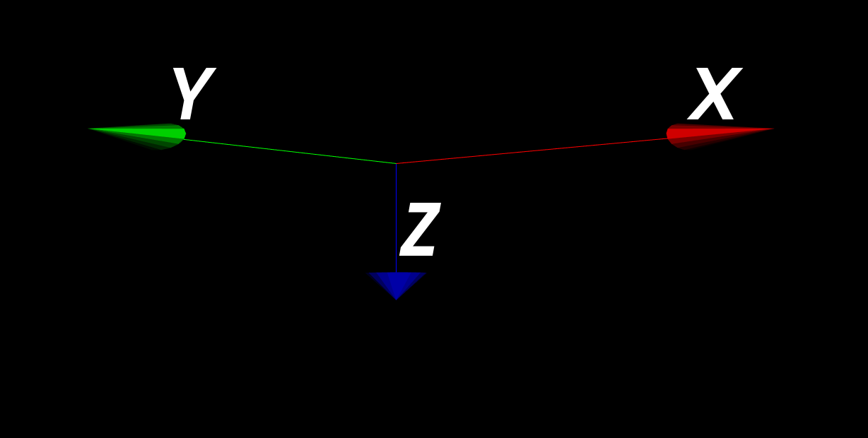
vtkSPtrNew( axes, vtkAxesActor );
axes->SetTotalLength( 1, 1, 1 ); // change length of three axis
axes->SetUserTransform( finalM );
double *scaleFactor = finalM->GetScale();
cout << "scaleFactor: " << scaleFactor[0] << ", " << scaleFactor[1] << ", " << scaleFactor[2] << endl;
vtkSPtrNew( renderer, vtkRenderer );
renderer->AddActor( axes );
renderer->SetBackground( 0, 0, 0 );
vtkSPtrNew( renderWindow, vtkRenderWindow );
renderWindow->AddRenderer( renderer );
vtkSPtrNew( renderWindowInteractor, vtkRenderWindowInteractor );
renderWindowInteractor->SetRenderWindow( renderWindow );
renderer->ResetCamera();
renderWindow->Render();
renderWindowInteractor->Start();
return EXIT_SUCCESS;
}
Define variable M =
![\[\begin{pmatrix} 2 & -2 & 0 \\ 0 & 0 & -1 \\ 2 & 2 & 0 \end{pmatrix}\]](https://www.weiy.city/wp-content/ql-cache/quicklatex.com-66bc2304f568138a4a0c953e41464ce9_l3.png "Rendered by QuickLaTeX.com")
eigenvalue decomposition
We have to review the eigenvalue decomposition.
If there is a constant value  and non-zero column vector
  has the relationship
  , we can get the new representation
  .
.
The eigenvalues are going to fill the diagonal, and the eigenvectors are going to form  .
.
![\[AX = \lambda X\]](https://www.weiy.city/wp-content/ql-cache/quicklatex.com-81b4f8cfdfff0ecf634538bfef77971c_l3.png "Rendered by QuickLaTeX.com")
![\[\lambda E X - A X = (\lambda E - A)X =0\]](https://www.weiy.city/wp-content/ql-cache/quicklatex.com-f8816aea14b9a581d9b8a66d47277c7c_l3.png "Rendered by QuickLaTeX.com")
When the eigenvalues polynomial is equal to 0, it’s called the eigenvalues equation of A.
![\[|\lambda E - A| = 0\]](https://www.weiy.city/wp-content/ql-cache/quicklatex.com-b88699a0775903bc21a524ef5ad5f334_l3.png "Rendered by QuickLaTeX.com")
For example, A =
![\[\begin{pmatrix} 1 & -2 \\ 1 & 4 \end{pmatrix}\]](https://www.weiy.city/wp-content/ql-cache/quicklatex.com-dbe073f108b106ae0b86a4947cbefe70_l3.png "Rendered by QuickLaTeX.com")
![\[|\lambda E - A| = \begin{vmatrix} \lambda - 1 & 2 \\ -1 & \lambda - 4 \end{vmatrix} = (\lambda - 1)(\lambda - 4) +2 = 0\]](https://www.weiy.city/wp-content/ql-cache/quicklatex.com-fb6dd0325eed9a535d0ccdb94bf668ea_l3.png "Rendered by QuickLaTeX.com")
Solve it, we get:  .
.
When  , we have:
![\[(\lambda E - A)X = \begin{pmatrix} 1 & 2 \\ -1 & -2 \end{pmatrix} \times \begin{pmatrix} x \\ y \end{pmatrix} = 0\]](https://www.weiy.city/wp-content/ql-cache/quicklatex.com-c9bb83c517979aef4b875d66cb525f82_l3.png "Rendered by QuickLaTeX.com")
Set X=1, we get Y = -0.5. So an eigenvector is (1, -0.5).
In the case  , we get the eigenvector(1, -1).
So we have :
![\[A = \begin{pmatrix} 1 & -2 \\ 1 & 4 \end{pmatrix} = \begin{pmatrix} 1 & 1 \\ -0.5 & -1 \end{pmatrix} \times \begin{pmatrix} 2 & 0 \\ 0 & 3 \end{pmatrix} \times \begin{pmatrix} 2 & 2 \\ -1 & -2 \end{pmatrix} = W \Sigma W^{-1}\]](https://www.weiy.city/wp-content/ql-cache/quicklatex.com-22ae78809eb5738b3240fc545e37ef05_l3.png "Rendered by QuickLaTeX.com")
singular value decomposition
A more popular decomposition way for matrix is singular value decomposition, SVD. It says,  . It can be proved by eigenvalue decomposition. SVD does not require the matrix to be decomposed as a square matrix. Let’s say our matrix A is an m x n matrix.
We can use SVD algorithm to decomposite the example’s matrix M.
// decomposition.
    double factors[3];
    auto matrix = finalM->GetMatrix();
    double U[3][3], VT[3][3];
    for( int i = 0; i < 3; ++i )
    {
        U[0][i] = matrix->GetElement( 0, i );
        U[1][i] = matrix->GetElement( 1, i );
        U[2][i] = matrix->GetElement( 2, i );
    }
    vtkMath::SingularValueDecomposition3x3( U, U, factors, VT );
    vtkSPtrNew( matrix_U, vtkMatrix3x3 );
    matrix_U->DeepCopy( (const double *)U );
    matrix_U->PrintSelf( std::cout, vtkIndent() );
    /*
    0.707107    -0.707107   0
    0   0   -1
    0.707107    0.707107    0
*/

    vtkSPtrNew( matrix_W, vtkMatrix3x3 );
    matrix_W->Identity();
    for( int i = 0; i < 3; ++i )
        matrix_W->SetElement( i, i, factors[i] );
    matrix_W->PrintSelf( std::cout, vtkIndent() );
    /*
    2.82843 0   0
    0   2.82843 0
    0   0   1
*/

    vtkSPtrNew( matrix_VT, vtkMatrix3x3 );
    matrix_VT->DeepCopy( (const double *)VT );
    matrix_VT->PrintSelf( std::cout, vtkIndent() );
    /*
    1   0   0
    0   1   0
    0   0   1
*/
So we get:

The interface finalM->GetScale(); returns singular values of original matrix.
